

Based on the study session transcript, which overrides the previous document, here is a summary of the confirmed topics for the exam.
Crucial Update from the Study Session: Contrary to the initial “Exam Requirements” document, the professor explicitly stated in the review session that formulas will be provided for the calculations, including the computational formulas for variance and correlation.
1. Variance ($s^2$) and Standard Deviation ($s$)
You are required to calculate these values to determine the components needed for correlation and regression. The transcript confirms that both the definitional and computational formulas are on the provided formula sheet.
- Definitional Formula: $$s^2 = \frac{\sum (X – \bar{X})^2}{N – 1}$$ Note: The standard deviation ($s$) is simply the square root of the variance.
- Computational Formula (Requested for Practice): The textbook provides the computational formula, which is useful because it reduces rounding errors by using raw scores rather than deviations. $$s^2 = \frac{\sum X^2 – \frac{(\sum X)^2}{N}}{N – 1}$$
- $\sum X^2$: Square each value first, then sum them.
- $(\sum X)^2$: Sum all values first, then square the total.
2. Pearson Correlation ($r$)
You must be able to calculate $r$ by hand. The transcript indicates that the computational formula is provided on the exam sheet.
- Definitional Formula: $$r = \frac{cov_{XY}}{s_x s_y}$$ (Covariance divided by the product of the standard deviations).
- Computational Formula (Requested for Practice): This formula allows you to calculate $r$ using the sums of raw scores, which corresponds to the “tabulation” method (columns for $X, Y, X^2, Y^2, XY$) described in the review session. $$r = \frac{N\sum XY – \sum X \sum Y}{\sqrt{[N\sum X^2 – (\sum X)^2][N\sum Y^2 – (\sum Y)^2]}}$$
3. Simple Linear Regression (Slope and Intercept)
You must calculate the slope and intercept to build the line of best fit: $\hat{Y} = b_0 + b_1X$ (or $\hat{Y} = a + bX$). The professor emphasized that while these formulas are provided, you must know how to populate them using the means and standard deviations you calculated earlier.
- Slope ($b_1$): $$b_1 = r \frac{s_y}{s_x}$$ (Correlation times the ratio of the standard deviations).
- Intercept ($b_0$): $$b_0 = \bar{Y} – b_1\bar{X}$$ (Mean of Y minus the Slope times the Mean of X).
4. Gauss-Markov Assumptions
You must know the three assumptions required for Ordinary Least Squares (OLS) to be the optimal estimator. The professor confirmed these are testing the properties of the residuals (errors), not the raw data.
- Normality: The residuals are normally distributed around a mean of zero.
- Homoskedasticity: The variance of the residuals is constant across all levels of X (equal variance).
- Independence: The residuals are independent of one another (no auto-correlation).
5. Model Equivalence (t-test vs. Regression)
You are expected to understand that the independent samples t-test (or two-sample t-test) is mathematically equivalent to a simple linear regression with a categorical predictor (binary X variable). The t-test is simply a specific case of the general linear model.
6. R-Squared ($R^2$)
The professor admitted he forgot to lecture on this topic. Consequently, the answer to the question regarding $R^2$ (the proportion of variance explained) will be provided on the formula sheet/test, essentially as a “free point”. You should still recognize that $R^2$ represents the proportion of variance in the outcome variable explained by the model.
The Gauss-Markov Theorem (GMT)
The Gauss-Markov Theorem provides the theoretical justification for using Ordinary Least Squares (OLS) as the method for estimating the parameters of a regression model. The theorem states that if a specific set of assumptions regarding the residuals (errors) of a model are met, the OLS algorithm yields the Best Linear Unbiased Estimators (BLUE).
This means that OLS estimates for the intercept ($b_0$) and slope ($b_1$) will have the smallest possible variance among all linear unbiased estimators, making them the optimal choices for minimizing error,.
The three critical assumptions required by the theorem are:
1. Normality of Residuals The residuals must be normally distributed with a mean of zero,.
- Concept: At every value of the predictor variable ($X$), the observed data points ($Y$) vary around the regression line. This variation (error) should follow a normal distribution centered on the line,.
- Visual Check: A histogram of residuals should look bell-shaped, and a Q-Q plot should show points falling along a straight diagonal line.
- Flexibility: While normality is an assumption, OLS is somewhat robust; minor violations are generally acceptable, but extreme violations can be problematic.
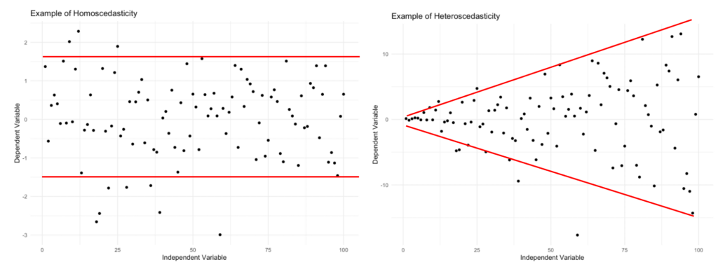
2. Homoskedasticity (Equal Variance) The residuals must have constant variance across all levels of the predictor variable ($X$),.
- Concept: The spread of the errors should be consistent regardless of whether $X$ is low or high. The conditional distribution of $Y$ at every value of $X$ should have the same variance ($\sigma^2$).
- Visual Check: When plotting fitted values against residuals, you should see a consistent cloud of dots. If you see a “cone shape” (where errors fan out and become larger as values increase), the assumption is violated.
3. Independence of Residuals The residuals must be independent of one another; the error for one observation should not predict the error for another,.
- Concept: The covariance between any two different error terms must be zero ($Cov(\epsilon_i, \epsilon_j) = 0$).
- Violations: This is often violated in time-series data (autocorrelation) or clustered data (e.g., students within the same classroom).
- Test: The Durbin-Watson test is used to check this assumption. A value of approximately 2 indicates independence; deviations from this suggest positive or negative correlation among residuals.
Model Equivalence
The course materials emphasize that “everything is regression”. Statistical tests commonly taught as distinct procedures, such as the t-test and ANOVA, are mathematically equivalent to linear regression models with categorical predictors.
1. The Independent Samples t-test as Linear Regression An independent samples t-test compares the means of two groups. This is identical to a Simple Linear Regression (SLR) where the predictor ($X$) is a binary categorical variable (dummy coded).
- Coding: One group is coded as $0$ (reference group) and the other as $1$ (comparison group).
- Intercept ($b_0$): In this regression, the intercept represents the mean of the reference group (where $X=0$).
- Slope ($b_1$): The slope represents the mean difference between the two groups. It is the amount added to the intercept to get the mean of the comparison group,.
- Equivalence: The $t$-statistic calculated for the slope in the regression output is numerically identical to the $t$-statistic from an independent samples t-test,.
2. ANOVA as Linear Regression Analysis of Variance (ANOVA) tests whether the amount of explainable variance (between groups) is significantly greater than the unexplainable random variance (within groups).
- Concept: ANOVA partitions the total variation ($SST$) into explainable variation ($SSR$) and unexplainable variation ($SSE$).
- F-Test: The F-statistic in a regression model serves the same purpose as the F-statistic in ANOVA. It tests if the model explains a significant proportion of the variance compared to the null model (the mean),.
- Multiple Regression: When a categorical variable has more than two levels, or when multiple predictors are used, Multiple Linear Regression (MLR) performs the same function as Factorial ANOVA, assessing main effects and interactions by partitioning variance,.