
The Breakdown
Here is a thorough review of the provided materials:
Important
- Variability – Refers to how spread out your scores are in the data. It can only be calculated when the dependent variable is measured on a continuous scale (interval or ratio) because it requires adding scores together and assumes the underlying property is continuous. It tells us the expected distance between every score and its average, and how much each individual score or sample mean represents the entire distribution or population.
- Accompanying Averages – Whenever an average is reported, a measure of variability must also be reported to indicate whether that average is a good or weak representation of the data.
- Interpreting Variability Magnitude – A very large variability suggests too much difference between subjects, meaning the average isn’t a good representation and may require increasing sample size or changing sampling/measurement. Conversely, very small variability indicates data is too close to the mean, implying insufficient sampling breadth and potential misrepresentation of the population.
- Range Calculation for Continuous Data – When data is on a continuous scale (ratio or interval), the range must consider “real limits”. The range is calculated as
(maximum score + 0.5) - (minimum score - 0.5)or simply(highest score - lowest score) + 1. If the data is discrete, real limits are not used, and the range is(X max - X min). - Limitation of Range – The range can provide a distorted picture of data spread because its calculation only uses the two extreme data points (highest and lowest scores), failing to account for the distribution of scores in between.
- Variance – An average measure of how far each unit is from the average, in squared units. Unlike the range, variance includes every single data point in its calculation.
- Sum of Squares (SS) – This is the total distance from the average obtained by squaring each deviation before adding them, which mathematically eliminates negative signs. SS represents the total amount of variation around the mean.
- Variance Formula for Samples (n-1) – For a sample variance (s²), the sum of squares (SS) is divided by
n-1(degrees of freedom). Thisn-1adjustment is crucial because sample variance typically underestimates the true population variance, making the sample variance an unbiased estimate of the population variance. - Standard Deviation – The average measure of how spread out the scores are around the average, in their original units of measurement. It is derived by taking the square root of the variance. A small standard deviation indicates scores are very close to the average (pointy or leptokurtic distribution), while a large standard deviation means scores are very spread out (flat or platykurtic distribution). Standard deviation is the measure typically reported in published research papers, not variance.
- Z-Scores – Z-scores transform original data into a new, comparable score, much like converting inches to centimeters. The shape of the distribution remains the same during this transformation, only the scale changes. Every single score in a sample or population can be transformed into a corresponding Z-score. Z-scores are critical for hypothesis testing and for comparing data measured on different scales.
- Z-Score Formulas (Sample vs. Population) – It is essential to choose the correct formula based on whether you are working with a sample or a population.
- Sample:
Z = (X - M) / S(score minus sample mean, divided by sample standard deviation). - Population:
Z = (X - μ) / σ(score minus population mean, divided by population standard deviation).
- Sample:
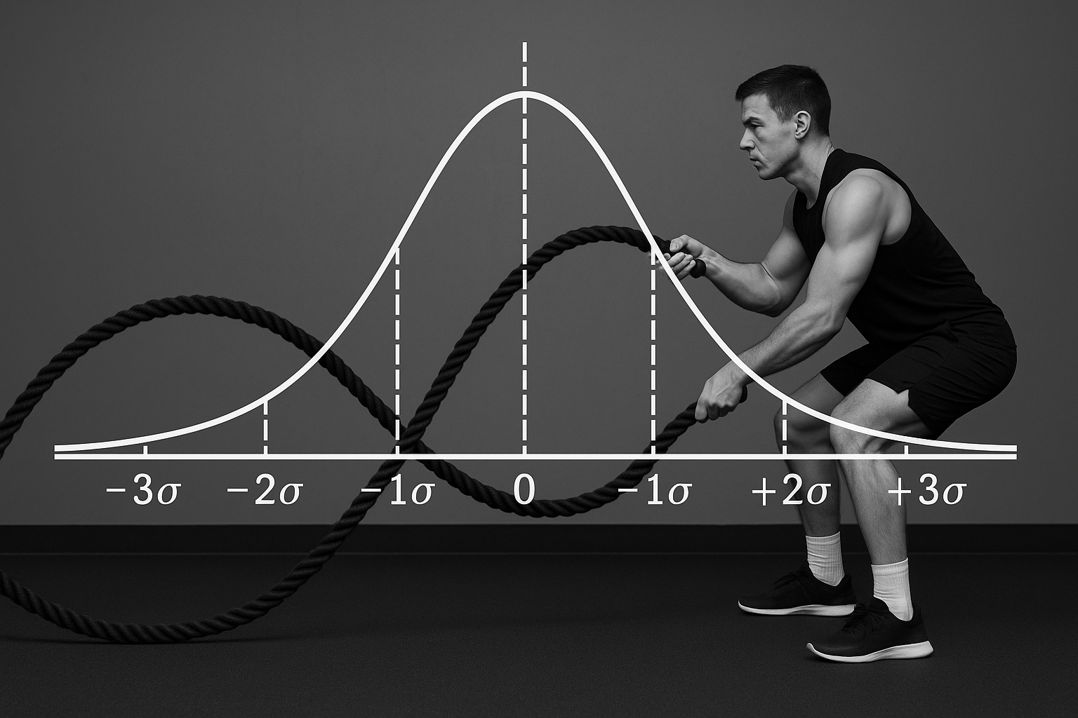
- Standard Normal Curve – This curve has an average (mean, μ) of 0 and a standard deviation (σ) of 1. The total area under this symmetrical curve is 1.00, with each half being 0.50. It allows us to determine where a particular score sits on the distribution and the probability of obtaining that score.
- Standard Deviation as Scale Movement – The standard deviation signifies that for every one standard score (or Z-score) movement on the standard normal curve, the original raw score scale moves by the value of the standard deviation.
Core Concepts
- Definition of Variability: Variability quantitatively describes the extent to which individual data points are spread out around the mean of a dataset.
- Goal of Variability Measurement: The primary objective is to obtain an average measure of how spread out the scores are within a dataset, akin to how the mean provides an average measure for central tendency.
- Visual Representation of Variability (Kurtosis): The shape of a distribution curve, specifically its kurtosis (mesokurtic for normal, platykurtic for flat, leptokurtic for pointy), visually conveys the variability of the data. Different shapes can have identical means but varying standard deviations, illustrating how variability provides additional insight beyond central tendency.
- Three Measures of Variability: The course focuses on three principal ways to quantify variability: the range, the variance, and the standard deviation.
- Real Limits Concept: For continuous data, real limits acknowledge the existence of decimal points between absolute numbers. These limits are considered when calculating the range to ensure accuracy.
- Sum of Squared Deviations (SS): This is a crucial intermediate step in calculating variance. Individual deviations of scores from the mean are squared before being summed to eliminate negative values, thereby allowing for a total measure of distance from the average.
- Degrees of Freedom (n-1) in Variance Calculation: The term
n-1(degrees of freedom) is used as a divisor when calculating sample variance to mathematically correct for the tendency of sample variance to underestimate the true population variance, thus yielding a more unbiased estimate. - Relationship between Variance and Standard Deviation: Variance represents the average spread of scores from the mean in squared units, making it less intuitive for interpretation. The standard deviation, derived by taking the square root of the variance, transforms this measure back into the original units of measurement, making it directly interpretable as an average distance from the mean.
- Z-score Transformation: This process involves converting raw scores from any continuous scale into a standardized Z-score. This transformation allows for comparing scores from different measurement scales on a common, standardized distribution (the standard normal curve), enabling a clearer understanding of a score’s position relative to its mean and other scores.
- Properties of the Standard Normal Curve: The standard normal curve is a symmetrical, bell-shaped distribution with a defined mean of 0 and a standard deviation of 1. It provides a framework for interpreting Z-scores and determining the proportion or percentage of scores that fall within specific ranges, aiding in probability assessment.
- Applications of Z-Scores: Beyond facilitating comparisons across different scales (e.g., entrance exams like MCAT, LSAT, GRE), Z-scores are fundamental for positioning an individual score within its distribution and are an important component in hypothesis testing.
Theories and Frameworks
- Standard Normal Curve / Standard Normal Distribution: A theoretical, bell-shaped, symmetrical distribution with a mean of 0 and a standard deviation of 1. It is used as a framework to understand and interpret data variability, particularly through the use of Z-scores, and to determine probabilities associated with scores.
Notable Individuals
- No notable individuals other than the instructor were mentioned in the provided source material.